Introduction
Now that the National League season has reached it’s conclusion for Southend United, I wanted to write one more data analysis piece looking at how we have performed in front of goal this season.
As we all know, the off-field situation at the club has defined our season, and there is a strong argument to suggest that had we been under normal circumstances, we would have finished higher up the table. Whilst this is true, I also believe that our ability in front of goal has contributed.
In this article, I will look at how we have performed in front of goal, provide an explanation of what the expected goals (xG) metric is, and explain the difference between pre-shot and post-shot xG.
Southend’s Expected Points
The below chart shows Southend’s performance compared to other clubs in the 2022/23 National League season for different metrics. The further each bar is to the right, the better we have performed in that particular metric. Don’t worry too much about the detail — there are just a few key metrics here that I want to mention, as I will detail below.
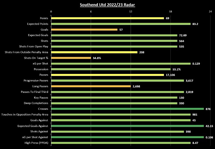
First of all, I want to compare our points to our number of expected points.
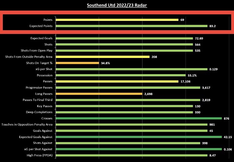
As you can see from the above chart, the number of points we picked up this season (69) is significantly lower than our number of expected points (83.2).
Expected points are calculated by taking each sides expected goals figures for every match to work out a probability for how likely each result was. For example, if in one particular match one side had accumulated a far higher expected goals figure than the other, they would gain more expected points than the other side. The expected points for each match are added up to give a total figure.
That means that the two metrics that can influence expected points are expected goals for, and expected goals against.
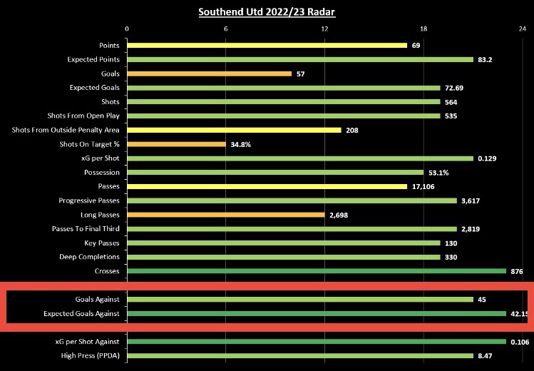
When we compare the number of goals we conceded (45) to our expected number (42.15) using the below chart, we can see that the two figures are fairly similar, so it doesn’t look like this has contributed a great deal to our under performance of expected points.
Next, when we compare our actual goals scored (57) to expected (72.69), we can quite clearly see a huge under performance in front of goal, using the below chart.
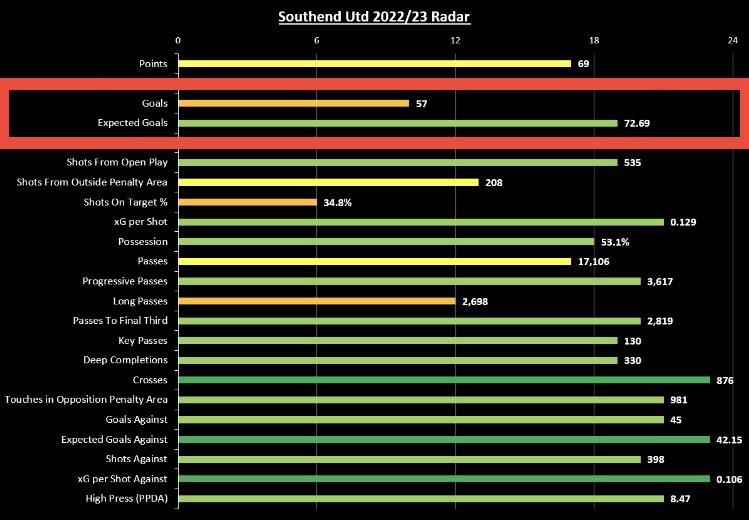
So, we’ve identified that we’ve scored less goals than we would’ve been expected to, but what exactly are expected goals and how are they calculated?
Expected Goals
Expected goals (xG) aims to assess the likelihood of scoring for every shot taken in each match. Different data providers have their own xG models, meaning there may be some differences to how they each work out expected goals, but for every shot, the xG model that I use from Wyscout calculates the probability to score based on things like shot location, and whether the shot was taken with the foot or head. The data models take into consideration a large number of shots from historical matches to predict the probability of every shot being scored.
Each shot is assigned a probability of how likely it is to result in a goal, from 0% (impossible to score) to 100% (impossible to miss). A shot with a 25% chance of scoring for example is assigned a value of 0.25. Penalties are assigned a fixed xG value of 0.76. These values are added up to give each side a total xG figure for every match, and can also be added to give a team/player total over a longer period of time.
Expected goals can easily be misused, and are much more effective when tracked over a period of time rather than in a one-off match. When we look at our xG from this season, as previously mentioned, we have under performed by around 15 goals.
Wyscout’s xG model also doesn’t take into consideration the position of opposing players. This means that two shots from similar areas of the pitch may be assigned similar xG values, even if one shot is taken with a clear sight of goal, and another is taken with multiple opposing players surrounding the striker, who may be able to block the shot. This may go some way to explaining why we have under performed compared to our xG.
So what are the reasons for teams under or over performing their xG? Finishing ability, goalkeeping performance and luck can all be contributing factors, and it’s usually a combination of all three.
This means that there’s an argument to suggest that we’ve just been really unlucky in front of goal this season, and if we keep on doing what we’ve been doing, eventually we’ll start to score more goals and match our xG.
There will be some truth to this. However I think there’s more to it than that, based on a couple of reasons which I will go through now.
First, by considering the amount of shots a side takes can provide another layer of context. For instance, if both sides accumulate an xG of 1.00 in a match, it may look like you’d expect the match to end 1-1. However, if one side achieves this figure by taking 20 shots all with an xG value of 0.05 (a 5% chance of scoring), and the other achieves it by having two shots with a 50% chance of scoring (0.50 xG), the side with fewer shots is more likely to win.
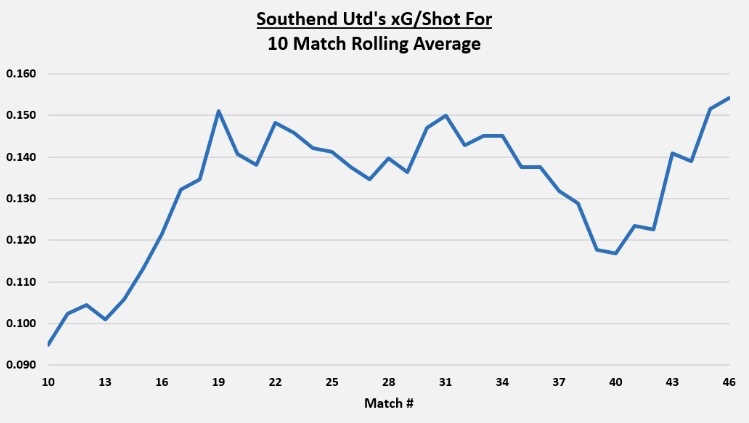
Earlier in the season I wrote about this (link to Twitter thread below), and found that after our first 10 matches we generally took lots of shots, but when you worked out the average probability of each of those shots being converted, it was very low. This resulted in a very low ‘xG per Shot’ value.
This wasn’t a problem all season however. From looking at the below graph you can see how, on a 10 match rolling average, we started the season with a very low ‘xG per Shot’ value, but this improved as the season went on, barring a drop off around the time of our seven match losing streak. I believe that the reintroduction of Jack Bridge to the side was critical to this improvement (link to Twitter thread also below).
The Difference Between Pre-Shot & Post-Shot xG
To understand the second reason for our under performance of xG, we need to understand the concept of post-shot xG.
As I have mentioned above, pre-shot xG (more commonly referred to as simply xG) measures the likelihood of each shot resulting in a goal. This is measured at the point the shot is taken, and doesn’t take into consideration the trajectory of the shot.
Where post-shot xG differs, is that only shots on target are included, with all blocked shots and shots off target automatically assigned a value of 0, as it’s impossible to score in these scenarios. Shot trajectory is also included, meaning we now know where the shot is heading.
So what are the benefits of using post-shot xG rather than simply normal pre-shot xG?
One benefit is that it helps to give a good indication of goalkeeping performance. If only shots on target are included in a post-shot xG model, we can see how many goals a goalkeeper would have been expected to concede based on the shots on target they have faced, if not for a save.
Another benefit is that we can get a better idea of finishing ability. This is because you can increase or decrease the likelihood of a shot being converted, when you compare the pre-shot xG and post-shot xG of any given shot. This may sound confusing, but I’ll try to explain further using an example.
In the below example from an away match this season, this shot from a Chesterfield player was assigned an xG value of 0.14 xG. This means that, at the point that the shot was taken, this was deemed to have a 14% chance of resulting in a goal.

Without knowing where the shot is heading, it may look fairly unlikely to be converted. Maybe it will be off target. Maybe the goalkeeper will save it.
The shot in question was in fact on target, hitting the post and going into the back of the Southend net.
When the shot trajectory is considered, the same shot was given a 0.51 post-shot xG (PSxG) value, meaning the shot would be expected to be scored 51% of the time.

Now we know that the shot is heading right for the corner of the goal and will be on target, it looks less likely the shot will be saved. As it’s in the corner, it’s a good finish, hence the higher PSxG value than xG.
When we compare Southend’s total post-shot xG this season (61.93) to our pre-shot xG (72.69), you can see a big difference. Once shot trajectory is considered, we would be expected to score fewer goals than if the probability was measured at the point our shots were attempted. This means that after shooting, we have actually reduced the likelihood of our shots being converted by around 10 goals, indicating poor finishing.
This PSxG figure of 61.93 is also much closer to the number of goals we actually scored (57), than our xG figure of 72.69.
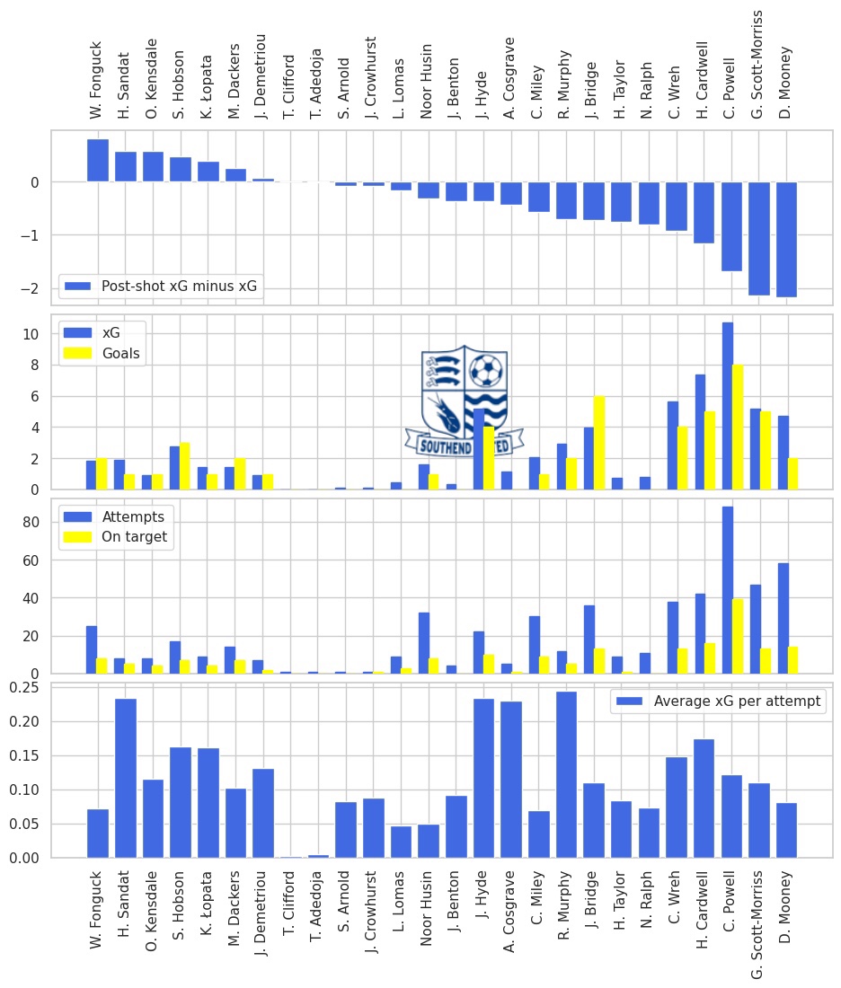
Using this below visualisation, at the top we can see that we don’t have many players who’s PSxG exceeds their xG — which would indicate good finishing — and most of the players we have that do are defenders, who obviously take fewer shots than our forward players.
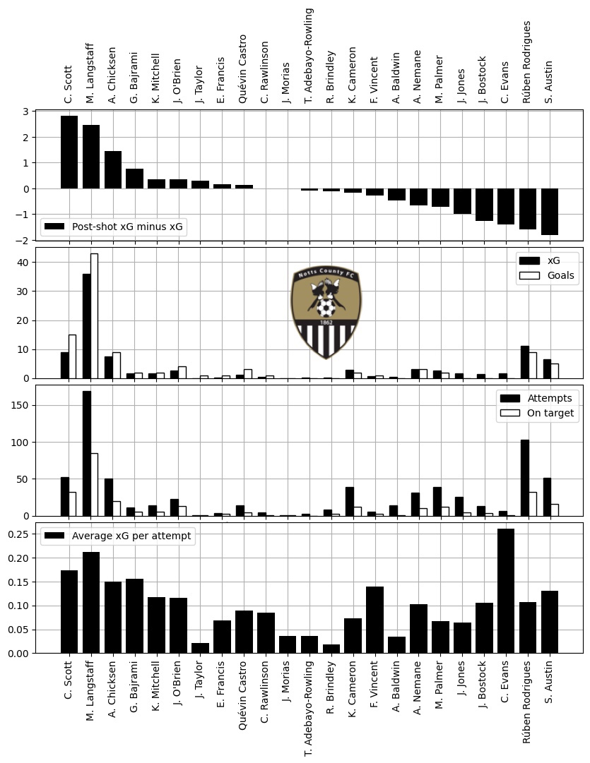
Compare that to Notts County for example, and they have more players who’s PSxG exceeds their xG, most notably forwards Macaulay Langstaff and Cedwyn Scott.

You must be logged in to post a comment.